f
(
x
)
=
c
o
s
(
x
)
+
s
i
n
(
2
x
)
2
Altra forma algebrica della funzione:
f
(
x
)
=
c
o
s
(
x
)
+
s
i
n
(
x
)
c
o
s
(
x
)
=
c
o
s
(
x
)
⋅
[
1
+
s
i
n
(
x
)
]
Campo di esistenza.
R
Proprietà geometriche.
È una somma di funzioni periodiche con periodo
2
π
e
π
. Il periodo è minimo comune multiplo dei due periodi, quindi ancora
2
π
.
Si può studiare la funzione tra 0 e
2
π
.
Intersezione con gli assi.
Radici.
f
(
x
)
=
0
→
c
o
s
(
x
)
⋅
[
1
+
s
i
n
(
x
)
]
=
0
→
{
c
o
s
(
x
)
=
0
1
+
s
i
n
(
x
)
=
0
→
x
A
=
π
2
,
x
B
=
3
2
π
,
le radici tra 0 e
2
π
.
Intercetta.
f
(
0
)
=
c
o
s
(
0
)
⋅
[
1
+
s
i
n
(
0
)
]
=
1
. C(0,1) è il punto d'intercetta.
Segno della funzione.
f
(
x
)
≥
0
→
c
o
s
(
x
)
⋅
[
1
+
s
i
n
(
x
)
]
≥
0
→
[
c
o
s
(
x
)
≥
0
]
⋅
[
s
i
n
(
x
)
≥
-
1
]
→
[
c
o
s
(
x
)
≥
0
]
→
[
0
,
π
2
]
∨
[
3
2
π
,
2
π
]
Asintoti.
Verticale. Nessun punto di discontinuità
Orizzontale.
l
i
m
x
→
±
∞
c
o
s
(
x
)
⋅
[
1
+
s
i
n
(
x
)
]
=
è una funzione oscillante e limitata
Obliqui. Nessun asintoto obliquo (anche la derivata è oscillante e limitata).
Punti stazionari.
f
'
(
x
)
=
d
d
x
[
c
o
s
(
x
)
⋅
[
1
+
s
i
n
(
x
)
]
]
=
-
s
i
n
(
x
)
+
c
o
s
(
2
x
)
=
-
s
i
n
(
x
)
+
1
-
2
⋅
s
i
n
2
(
x
)
=
-
2
⋅
s
i
n
2
(
x
)
-
s
i
n
(
x
)
+
1
f
'
(
x
)
=
0
→
2
⋅
s
i
n
2
(
x
)
+
s
i
n
(
x
)
-
1
=
0
→
s
i
n
(
x
)
=
-
1
±
1
+
8
4
=
-
1
±
3
4
→
{
s
i
n
(
x
)
=
-
1
s
i
n
(
x
)
=
1
2
→
{
x
B
=
3
2
π
x
D
=
1
6
π
,
x
E
=
5
6
π
Tre punti stazionari tra 0 e
2
π
. Il primo corrispondente a una radice
Gli altri due hanno ordinata:
f
(
x
D
)
=
c
o
s
(
1
6
π
)
⋅
[
1
+
s
i
n
(
1
6
π
)
]
=
3
2
(
1
+
1
2
)
=
3
4
⋅
3
e
f
(
x
E
)
=
c
o
s
(
5
6
π
)
⋅
[
1
+
s
i
n
(
5
6
π
)
]
=
-
3
2
(
1
+
1
2
)
=
-
3
4
⋅
3
Il segno della derivata prima.
-
2
⋅
s
i
n
2
(
x
)
-
s
i
n
(
x
)
+
1
≥
0
→
2
⋅
s
i
n
2
(
x
)
+
s
i
n
(
x
)
-
1
≤
0
→
-
1
≤
s
i
n
(
x
)
≤
1
2
→
0
≤
x
≤
π
6
∨
5
6
π
≤
x
≤
2
π
in
x
=
π
6
un massimo
D
(
π
6
,
3
4
⋅
3
)
in
x
=
5
6
π
un minimo
E
(
5
6
π
,
-
3
4
⋅
3
)
in
x
=
3
2
π
un flesso a tangente orizzontale
A
(
π
2
,
0
)
Curvature.
f
'
'
(
x
)
=
d
d
x
{
-
2
⋅
s
i
n
2
(
x
)
-
s
i
n
(
x
)
+
1
}
=
-
4
⋅
c
o
s
(
x
)
⋅
s
i
n
(
x
)
-
c
o
s
(
x
)
=
-
c
o
s
(
x
)
⋅
[
s
i
n
(
x
)
+
1
]
f
"
(
x
)
=
0
→
-
c
o
s
(
x
)
⋅
[
s
i
n
(
x
)
+
1
]
=
0
→
{
c
o
s
(
x
)
=
0
s
i
n
(
x
)
+
1
=
0
→
{
c
o
s
(
x
)
=
0
s
i
n
(
x
)
=
-
1
→
{
x
A
=
π
2
,
x
B
=
3
2
π
x
B
=
3
2
π
Tutti i flessi in punti già noti (A e B ). In A flesso a tangente obliqua discendente e in B flesso a tangente orizzontale.
Il segno della derivata seconda.
-
c
o
s
(
x
)
⋅
[
s
i
n
(
x
)
+
1
]
≥
0
→
(
c
o
s
(
x
)
≤
0
)
⋅
(
s
i
n
(
x
)
≥
-
1
)
→
(
π
2
≤
x
≤
3
2
π
)
L'equazioni della retta del flesso a tangente obliqua:
y
f
l
e
x
(
x
)
=
f
'
(
x
A
)
⋅
(
x
-
x
A
)
+
f
(
x
A
)
=
[
-
2
⋅
s
i
n
2
(
π
2
)
-
s
i
n
(
π
2
)
+
1
]
⋅
(
x
-
π
2
)
=
-
2
⋅
(
x
-
π
2
)
=
-
2
x
+
π
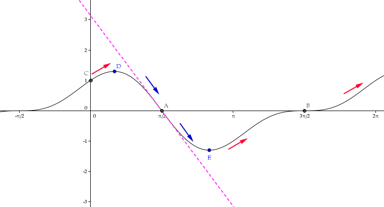
Qui di seguito il grafico finale della funzione.